Power-of-two padding
In my previous post, I wrote about using FFTs to compute a full convolution. If the vector x has $K$ points and the vector h has $L$ points, then the convolution of x and h has $K+L-1$ points. FFTs can be used to compute this convolution, but only if x and h are zero-padded to have at least $K+L-1$ points in the FFT computation.
Early in my career, the commonly available FFT algorithms, which were usually written in Fortran, were limited to computing FFT with transforms that were powers of two. Because of this limitation, using FFTs to compute convolution required zero-padding to the smallest power of two that was greater than or equal to $K+L-1$ . Here’s how that might look in MATLAB code.
x = [1 -1 0 4];
h = [1 0 -1];
K = length(x);
L = length(h);

N = K + L - 1
N = 6
Np = 2^nextpow2(N)
Np = 8
X = fft(x,Np);   % Computes Np-point zero-padded FFT
H = fft(h,Np);   % Computes Np-point zero-padded FFT

Y = ifft(X .* H);
y = Y(1:N)
y = 1x6
1.0000   -1.0000   -1.0000    5.0000         0   -4.0000
Small-primes padding
More than 20 years ago now, I integrated the FFTW library into MATLAB. FFTW, or “Fastest Fourier Transform in the West,” won the 1999 J. H. Wilkinson Prize for Numerical Software. I spent a long time deep in the FFTW documentation at the time, and this statement caught my attention: “The standard FFTW distribution works most efficiently for arrays whose size can be factored into small primes (2, 3, 5, and 7), and otherwise it uses a slower general-purpose routine.”
This observation suggests the interesting possibility of using transform lengths are powers of 2, 3, 5, and 7, instead of using only transform lengths that are powers of 2.
Here is a function that computes a transform length based on this idea.
function np = transformLength(n)
    np = n;

    while true
        % Divide n evenly, as many times as possible, by the factors 2, 3,
        % 5, and 7.
        r = np;
        for p = [2 3 5 7]
            while (r > 1) && (mod(r, p) == 0)
                r = r / p;
            end
        end

        if r == 1
            % If the result after the above divisions is 1, then we have found
            % the desired number, so break out of the loop.
            break;
        else
            % np has one or more prime factors greater than 7, so try the
            % next integer.
            np = np + 1;
        end
    end
end
Suppose n is 37, a prime number. The next power of 2 is 64. The next number whose largest prime factor 7 or less, on the other hand, is 40.
n = 37;
np = transformLength(n)
np = 40
factor(np)
ans = 1x4
     2     2     2     5
2-D performance comparisons
To see how different padding strategies affect performance, I will set up some different FFT-based 2-D convolution functions and measure their execution time for different input sizes. Here is function that zero-pads only to the minimum amount required, $K+L-1$ .
function C = conv2_fft_minpad(A,B)
    [K1,K2] = size(A);
    [L1,L2] = size(B);
    N1 = K1 + L1 - 1;
    N2 = K2 + L2 - 1;

    C = ifft2(fft2(A,N1,N2) .* fft2(B,N1,N2));
end
Let’s measure the time required to convolve a 1170x1170 input with a 101x101 input. The output will be 1271x1271, and 1271 has prime factors 31 and 41.
A = rand(1170,1170);
B = rand(101,101);
f_minpad = @() conv2_fft_minpad(A,B);
timeit(f_minpad)
ans = 0.0329
Here is a function that zero-pads to the next power of 2. (The next power of 2 above 1271 is 2048.)
function C = conv2_fft_pow2pad(A,B)
    [K1,K2] = size(A);
    [L1,L2] = size(B);
    N1 = K1 + L1 - 1;
    N2 = K2 + L2 - 1;
    N1p = 2^nextpow2(N1);
    N2p = 2^nextpow2(N2);

    C = ifft2(fft2(A,N1p,N2p) .* fft2(B,N1p,N2p));
    C = C(1:N1,1:N2);
end
Repeat the timing experiment using this second padding method:
f_pow2pad = @() conv2_fft_pow2pad(A,B);
timeit(f_pow2pad)
ans = 0.0553
So, power-of-2 padding is not helping in this case. The fact that power-of-2 padding is slower than using a transform length with relatively high prime factors represents a sea change from the way FFT computations in MATLAB performed prior to 2004, which is when MATLAB started using FFTW.
Can small-primes padding do better?
function C = conv2_fft_smallprimespad(A,B)
    [K1,K2] = size(A);
    [L1,L2] = size(B);
    N1 = K1 + L1 - 1;
    N2 = K2 + L2 - 1;
    N1p = transformLength(N1);
    N2p = transformLength(N2);

    C = ifft2(fft2(A,N1p,N2p) .* fft2(B,N1p,N2p));
    C = C(1:N1,1:N2);
end
Run the timing again with the small-primes pad method:
f_smallprimespad = @() conv2_fft_smallprimespad(A,B);
timeit(f_smallprimespad)
ans = 0.0230
Yes, the convolution function using the small-primes method runs about 45% faster for this case.
Now let’s compare the results for a range of sizes.
nn = 1100:1200;
t_minpad = zeros(size(nn));
t_pow2pad = zeros(size(nn));
t_smallprimespad = zeros(size(nn));
for k = 1:length(nn)
    n = nn(k);
    A = rand(n,n);
    t_minpad(k) = timeit(@() conv2_fft_minpad(A,B));

    t_pow2pad(k) = timeit(@() conv2_fft_pow2pad(A,B));

    t_smallprimespad(k) = timeit(@() conv2_fft_smallprimespad(A,B));
end
Plot the results.
plot(nn,t_minpad,nn,t_pow2pad,nn,t_smallprimespad)
ax = gca;
ax.YLim(1) = 0;
legend(["min padding","power-of-2","small-primes"],...
    Location="southeast")
title("Execution time, nxn convolution with 101x101")
xlabel("n")
ylabel("time (s)")
grid on
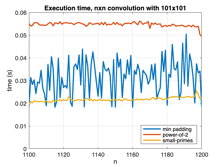
While this is admittedly not anything like a comprehensive performance study, it does suggest that:
- There is no longer a reason to do power-of-2 padding for 2-D convolution problems.
- Small-primes padding is almost always faster that minimum-length padding, even when considering the extra steps needed (computing the transform length and cropping the output of
ifft2. In a few cases, it is about the same or just slightly worse.
In my next post in this series, I plan to investigate a possible way to speed up the computation of the small-primes transform length.